python3 csv

Posted on 2018-06-24 | In notes.code

python3 输入输出csv文件的2种形式


import csv

def testCSVWriterReader():
    with open('csvtest.csv','w',newline='') as  cf:
        cw = csv.writer(cf,delimiter=',')
        cw.writerow(['aa','bb','cc'])
        cw.writerow(["aa"]*5+['ff'])
    cf.close()

    with open('csvtest.csv','r') as  f:
        cr = csv.reader(f,delimiter=',')
        for row in cr:
            print(row)
            for d in row:
                print(d,' ')
    f.close()

def testCSVDic():
    with open('csv_dict.csv','w') as  cf:
        csvhead = ['id','title']  # write head
        writer = csv.DictWriter(cf,fieldnames=csvhead)
        writer.writeheader();
        writer.writerow({'id': '1', 'title': 'aa'})
        writer.writerow({'id': '2', 'title': 'bb'})

    with open('csv_dict.csv') as  cf:
        reader = csv.DictReader(cf)
        for row in  reader:
            print(row['id'],row['title'])



print('testing writer and reader for csv file......')
testCSVWriterReader()

print('testing dic writer and dic reader for csv file..... ')
testCSVDic()

实体融合ER工具介绍

Posted on 2018-03-26 | In 调研

Dedupe

Github地址：https://github.com/dedupeio/dedupe
Dedupe，基于python的ER工具包。结合试用机器学习、主动学习等技术在结构化数据集上实现快速去重（de-duplication）和实体识别（entity resolution）。

记录相似性的衡量：string metric，实际采用Affine Gap Distance（Hamming distance的一个变种）。
属性逐步比较。与直接比较整条记录相比，可以为不同属性设置不同权重。比如地址去重任务中，电话号码可能比其他属性更为重要。
主动学习用来学习属性权重：人工标注难以判断的记录对（机器判断匹配可能性在50%附近的2条记录），然后机器重新学习属性权重。
使用多种Blocking技术并组合blocking规则以减少判断次数。包括属性，token，相同3个前缀字符，相同5个前缀字符，相同的7个前缀字符，4-gram，6-gram及倒排索引blocks等。
hierarchical clustering with centroid linkage聚类算法用于将不同的匹配对聚成类以表示一个实体。

Limes

Github地址：https://github.com/dice-group/LIMES
为Entity linking设计的框架，支持超大规模级实体链接。

时间优化。Plan技术决定哪些任务优先执行，发现任务之间的中间依赖关系以过滤任务，而非独立执行任务。Plan技术能大量减少执行时间。
支持海量的匹配规则，包括字符串，数值，拓扑及时序相似性矩阵度量及自定义距离计算模型
与暴力方法相比，Limes不会损失任何匹配精度但能显著减少匹配操作的数量。

在matlab使用libsvm

Posted on 2017-12-25 | In notes.tools

[heart_scale_label, heart_scale_inst] = libsvmread('heart_scale');
model = svmtrain(heart_scale_label, heart_scale_inst, '-c 1 -g 0.07 -b 1');
[predict_label, accuracy, prob_estimates] = svmpredict(heart_scale_label, heart_scale_inst, model, '-b 1');

label：n*1
data：n*d

在matlab中安装libsvm

Posted on 2017-12-23 | In notes.tools

参考http://blog.csdn.net/chensheng312/article/details/73195158

问题1: 未找到支持的编译器或 SDK。您可以安装免费提供的 MinGW-w64 C/C++ 编译器；请参阅安装 MinGW-w64 编译器。有关更多选项，请访问
http://www.mathworks.com/support/compilers/R2016a/win64.html

解决方案：http://blog.csdn.net/desire121/article/details/60466845

1.新建环境变量 MW_MINGW64_LOC，设置为TDM-GCC-64的安装位置（‘D:\mingw-w64\mingw-w64\x86_64-4.9.2-posix-seh-rt_v3-rev1\mingw64\’）,路径最后不要加bin
2.在MATLAB环境下执行setenv(‘MW_MINGW64_LOC’,folder)。folder为TDM-GCC的安装位置，要加单引号；
3.重启MATLAB

mex -h
mex CFLAGS="\$CFLAGS -std=c99" -largeArrayDims libsvmread.c -v

使用 -v 参数展示详细模式，可以看到需要查找的编译器

问题2: gcc: error: -fexceptions: No such file or directory
解决方案：https://github.com/cjlin1/libsvm/issues/55
将make.m文件下的所有的CFLAGS都替换成COMPFLAGS

爬虫及解析

Posted on 2017-12-22 | In notes.tools

师弟写的爬虫及解析工具
temme

Sparse Autoencoder

Posted on 2017-12-17 | In notes.deeplearning

Tutorial of Unsupervised Feature Learning and Deep Learning by Andrew Ng

Neural Networks

activation function:

sigmoid function: 值域[0,1]
\begin{equation}
f(z) = \frac{1}{1+\exp(-z)}
\end{equation}

一阶导数为：$f’(z) = f(z)(1-f(z))$

tanh function (hyperbolic tangent) 双曲正切函数: 值域[ − 1,1]

\begin{equation}
f(z) = \tanh(z)=\frac{e^z-e^{-z}}{e^z+e^{-z}}
\end{equation}

一阶导数为：$f’(z) = 1-(f(z))^2$

Neural Network model

“feedforward neural network”
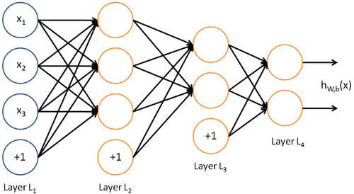
input layer $\to$ hidden layer $\to$ output layer

每层的神经元数量不计bias unit（bias unit对应intercept term，y=Wx+b 中的b）

设神经网络有$n_l$层，则图中 input layer （记为$L_1$,3 input units） $\to$ hidden layer ($L_2$,3 hidden units; $L_3$,2 hidden units) $\to$ output layer （记为$L_{n_l}$,2 output units）

第$l$ 层对应的参数为$W^l,b^l$，则

\begin{equation}
z^{l+1} = W^l a^l+b^l
\end{equation}

\begin{equation}
a^{l+1} = f(z^{l+1})
\end{equation}

$a^{l+1}$是一个向量，代表第$l+1$层的activation。其中$a^1$是输入x，$a^{n_l}$为输出y

feedforward neural network, the connectivity graph does not have any directed loops or cycles

Backpropagation Algorithm

反向传播算法从输出层开始，反向计算每个节点的残差，并用这些残差计算代价方程对每一个参数的偏导数。

数学原理

中文译者有给出数学证明

Gradient checking and advanced optimization

Autoencoders and Sparsity

Visualizing a Trained Autoencoder

Sparse Autoencoder Notation Summary

Deep Feedforward Networks

Posted on 2017-12-17 | In notes.deeplearning

Deep feedforward networks, 也称 feedforward neural networks, 或 multi-layer perceptrons (MLPs)。

MLP用来近似函数，信息从x，经过中间层计算，最后到y。如果一个扩展feedforward neural networks，使它包含feedback，则称为recurrent neural networks

有约束最优化方法(Constrained Optimization)

Posted on 2017-12-07 | In notes.math

unconstrained optimization: maximize or minimize a function $f(x)$ over all possible values of x
constrained optimization: find the maximal or minimal value of $f(x)$ for values of x in some set $\mathbb{S}$. 集合$\mathbb{S}$内的点称之为 feasible points

方法：

simply to modify gradient descent taking the constraint into account. （比如search only over step sizes that yield new x points that are feasible）
构造一个无约束最优化问题使得解能映射回原来的有约束最优化问题。

拉格朗日乘子法和KKT条件

参考深入理解拉格朗日乘子法（Lagrange Multiplier) 和KKT条件

拉格朗日乘子法(Lagrange Multiplier)和KKT(Karush-Kuhn-Tucker)条件是求解约束优化问题的重要方法。首先用等式约束和不等式约束来描绘集合$\mathbb{S}$。在有等式约束时使用拉格朗日乘子法，在有不等约束时使用KKT条件（KKT条件是拉格朗日乘子法的泛化）。只有当目标函数为凸函数时，使用这两种方法才保证求得的是最优解。

通常需要求解的最优化问题

无约束优化问题
$\min ~ f(x)$
有等式约束的优化问题

\begin{align}
\min & ~ f(x) \nonumber \\
s.t. & ~ h_i(x) = 0, i=1,…,m \label{problem_math}
\end{align}

有不等式约束的优化问题
\begin{align}
\min & ~ f(x) \nonumber \\
s.t. & ~ g_i(x) \le 0; i = 1,…,n \nonumber \\
& ~ h_j(x) = 0, j=1,…,m \label{problem_math2}
\end{align}

优化方法。

无约束优化问题

Fermat定理，即使用求取f(x)的导数，然后令其为零，可以求得候选最优值，再在这些候选值中验证；如果是凸函数，可以保证是最优解。

有等式约束的优化问题：拉格朗日乘子法

拉格朗日乘子法（Lagrange Multiplier) ，即把等式约束$h_i(x)$用一个系数与$f(x)$写为一个式子，称为拉格朗日函数，而系数称为拉格朗日乘子。通过拉格朗日函数对各个变量求导，令其为零，可以求得候选值集合，然后验证求得最优值。

the generalized Lagrangian or generalized Lagrange function is:

$L(x,\alpha) = f(x) +\sum_{i=1}^m \alpha_i h_i(x)$

或向量形式

$L(x,\alpha) = f(x) + \alpha h(x)$

这里把$\alpha$和$h(x)$视为向量形式，$\alpha$是横向量，h(x)为列向量

求解方法：对Lagrangian函数分别对$\alpha$ 和 $x$ 求导数，并令导数为0，得到$\alpha$ 和 $x$

$\nabla_x L(x,\alpha) = 0$ $\nabla_\alpha L(x,\alpha) = 0$

有不等式约束的优化问题：KKT条件

引入KKT multipliers，$\alpha$和$\lambda$,其中，$\alpha_i \ne 0$, $\lambda_j \ge 0$
向量形式：

$L(x,\alpha,\lambda) = f(x) + \alpha h(x)+\lambda g(x)$

KKT条件是说最优值必须满足以下条件：

$L(x,\alpha, \lambda)$对x求导为零；
$h(x) = 0$
$\lambda g(x) = 0$

原理推导看拉格朗日乘子法和KKT条件

无约束最优化方法

Posted on 2017-12-07 | In notes.math

unconstrained optimization method.

marked. 有时间再整理。

梯度下降法

最速下降法(Gradient Descent Method)使用梯度。

牛顿法

使用Hessian matrix

拟牛顿法（Quasi-Newton Methods）

不再直接计算hessian矩阵, 而是每一步的时候使用梯度向量更新hessian矩阵的近似

共轭方向法

共轭梯度法

直接法

不需要函数导数信息的方法，通过试算来寻找优化方向。它的优势在于对函数没有可微假设。劣势是收敛速度往往很慢。。

univariate search technique

单纯形法

Numerical Computation in deep learning

Posted on 2017-12-05 | In notes.math

update estimates of the solution via an iterative process (通过迭代过程逐步逼近解，而analytically deriving a formula providing a symbolic expression for the correct solution.)

Overflow and Underflow

rounding error：数值在计算机中存储时产生精度方面的误差，包含

underflow。数字接近0
overflow。数字接近正无穷大或负无穷大。

因此设计函数时要求 be stabilized against underflow and overflow

Poor Conditioning

输入的微小变化会引起计算结果的剧烈变化，即Poor Conditioning。

考虑$AX=b$，如果系统的解对系数矩阵A或b太敏感，（一般系数矩阵A和b是从实验数据里面估计得到，存在误差），方程组系统就是ill-conditioned。否则就是well-condition系统。

condition number：衡量ill-condition系统的可信度，衡量输入发生微小变化时，输出会发生多大的变化。也就是系统对微小变化的敏感度。

condition number值小（在1附近）：well-conditioned
condition number值大（远大于1）：ill-conditioned. 输出结果可靠性不高。

（L2范数有助于处理 condition number不好的情况下矩阵求逆很困难的问题）。

如果方阵A非奇异，则condition number定义为：
\begin{equation}
\kappa (A) = ||A|| ||A^{-1}||
\end{equation}

如果方阵A奇异，那么A的condition number正无穷大.

设函数$f(x) = A^{-1}x$, 方阵有特征分解。则condition number为：
\begin{equation}
\kappa (A) = \max_{i,j} |\frac{\lambda_i}{\lambda_j}|
\end{equation}

条件数即 the ratio of the magnitude of the largest and smallest eigenvalue.

Gradient-Based Optimization

Jacobian and Hessian Matrices

Jacobian矩阵和Hessian矩阵写得很好。

雅可比矩阵

假设$f: R^n \to R^m$是一个从欧式n维空间转换到欧式m维空间的函数. 这个函数$f(x) \in \mathbb{R}^m$由m个实函数组成: $f_1(x_1,…,x_n), …, f_m(x_1,…,x_n)$. 这些函数的偏导数(如果存在)可以组成一个m行n列的矩阵, 这就是所谓的雅可比矩阵：

$J=[\frac{\partial f}{\partial x_1},...,\frac{\partial f}{\partial x_n}]=\left[ \begin{matrix} \frac{\partial f_1}{\partial x_1} & \cdots & \frac{\partial f_1}{\partial x_n} \\ \vdots &\ddots & \vdots \\ \frac{\partial f_m}{\partial x_1} & \cdots & \frac{\partial f_m}{\partial x_n} \\ \end{matrix} \right]$

(这个矩阵的第i行是由梯度函数的转置$f_i(i=1,…,m)$表示的)

海森Hessian矩阵

the Hessian is the Jacobian of the gradient
(我的理解是对雅可比矩阵的某一行再做一次雅可比)

设函数$f(x_1,x_2,…,x_n)$,如果$f$的所有二阶导数都存在, 那么$f$的海森矩阵即：

$H(f)=\left[ \begin{matrix} \frac{\partial^2 f}{\partial x_1^2} & \frac{\partial^2 f}{\partial x_1 \partial x_2} & \cdots & \frac{\partial^2 f}{\partial x_1 \partial x_n} \\ \frac{\partial^2 f}{\partial x_2 \partial x_1} & \frac{\partial^2 f}{\partial x_2^2} & \cdots & \frac{\partial^2 f}{\partial x_2 \partial x_n} \\ \vdots & \vdots & \ddots & \vdots \\ \frac{\partial^2 f}{\partial x_n \partial x_1} & \frac{\partial^2 f}{\partial x_n \partial x_2} & \cdots & \frac{\partial^2 f}{\partial x_n^2} \\ \end{matrix} \right]$

Hessian matrix is real and symmetric，we can decompose it into a set of real eigenvalues and an orthogonal basis of eigenvectors.

判断极大值以及极小值

二阶导数用于判断函数critical point是否极大值/极小值：（一阶导数$f0(x) = 0$的点为 critical points 或 stationary points）

$f’(x) = 0, f’’(x) > 0 $ $x$ 局部最小值
$f’(x) = 0, f’’(x) < 0 $ $x$ 局部最大值
$f’(x) = 0, f’’(x) = 0 $ $x$ may be a saddle point(鞍点), or a part of a flat region.

多维情况下，使用Hessian matrix的特征分解：

Hessian is positive definite (all its eigenvalues are positive), the point is a local minimum
Hessian is negative definite (all its eigenvalues are negative), the point is a local maximum
at least one eigenvalue is positive and at least one eigenvalue is negative, we know that x is a local maximum on one cross section of f but a local minimum on another cross section. (a saddle point)

最优化方法

When the Hessian has a poor condition number, gradient descent performs poorly. 使用Hessian matrix to guide the search，最简单的一种是Newton’s method（基于2阶形式的泰勒展开）

first-order optimization algorithms：use only the gradient，比如 gradient descent
second-order optimization algorithms：use the Hessian matrix，比如 Newton’s method

弱限制条件：限制函数满足Lipschitz continuous or have Lipschitz continuous derivatives. quantify our assumption that a small change in the input made by an algorithm such as gradient descent will have a small change in the output.

强限制条件：Convex optimization. 只能应用于convex functions—functions for which the Hessian is positive semidefinite everywhere. 在deep learning中使用率不高。